US Treasury Cherry Picking

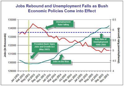
This is a nice example of cherry picking from a recent US Treasury Department press release. (Click for larger image) . In this case, the selection of the starting date, the scaling for the Y axes, and a pair of cooperating factors creates a strong impression of an economy that is going gangbusters and directly helping the ordinary working person.

Contrast this with the EPI talking points that we mentioned in our previous post that highlight a fairly lengthy list of the less than rosy things happening in the lives of American workers.

Picking a starting date near the peak for unemployment percent and near the low point for total jobs creates a different impression than if these same two factors had been viewed since 2000 or 1995 or 1990 or 1980. If you want to understand what's is happening with these two important metrics and to think about what it might mean, these other starting times will surely be instructive to your deliberations.

There is more going on here than just cherry picking. There is a strong push in this graphic to imply that there is powerful cause and effect relationship at work that is driving these numbers. Notice the vertical dotted yellow line for May 2003, the Green Text Box telling us "President Bush Signs Jobs and Growth Act (May 2003)", and the title linking the changes in these two factors to this specific President Bush action. Perhaps there is some relationship between that action and the visible results, but there is nothing in the graph or in the accompanying text of this press release that sheds light on how these two are in fact linked. The text box could equally well have said "Mission Accomplished (May 2003)".

Finally, the dotted blue line showing the average unemployment percentage from 1960-2005 is a great example of inappropriate use of averages and involves cherry picking of the starting and ending date. A very different blue line would have resulted from using the average unemployment from 1995-2000.

How can you protect yourself from Extremes of Cherry Picking? Here is how I would appraoch it.
a) look at the entire data time series yourself for each important factor - going back to at least 1980 in this case
b) zoom in and out on different time periods to grasp a fuller sense of the trends at work - include 1980-2005, 1990 through 2005, 1995 through 2005, 2000 through 2005
c) look at all the important factors - not just the ones that support your theory - in this case, the EPI datazone referenced in the previous post could be a good place to start. Once you have looked at this rather large set of factors, take a step back and think if there are any other factors that may have been left out.
d) adjust scaling as needed
e) look at different combinations of variables together
f) if you want to link the timing of specific events (e.g. the impact of Hurricane Katrina) or actions to what you see in the trends, create a list of the ones you think are most relevant.
g) try comparing different time periods - e.g. 1995 to 2000 compared to 2000-2005 with the factors that you consider the most important.

Economic Policy Institute Datazone

Another way to get a sense of the key factors that are at work and determine how well our economy is doing is to take a look at National Data from the EPI Datazone. Many more factors are available for review either by subcategory such as unemployment rates, or by downloading a spreadsheet with all the time series data for all the factors.

There are many more factors presented on the reference web page than were included in the article noted in our previous post - How is Our Economy Doing?

The one key thing that is missing is some way to make it easy for the lay person to quickly view all the the key factors, one at at a time, in an easy to ready trend graphic display .

A key goal of this blog is to help us move in the direction of ready reusability and we will be returning to this them in future posts.

How is Our Economy Doing?

How is Our Economy Doing? What are the Key Factors?

"What's wrong with the economy?" by Economic Policy Instute (EPI) President Lawrence Mishel and Policy Director Ross Eisenbrey addresses these very questions. Hat tip to Brad DeLong via Max Sawicky.

Mishel and Eisenbrey sketch the highlights of a range of key factors. Taken collectively, these can help us formulate a picture in our mind -- one that lets us gauge just how well our economy is doing.

These factors include:

Inflation-adjusted hourly wages
Inflation-adjusted weekly wages
Corporate profits
Productivity
Median household income (inflation-adjusted)
Indebtedness of U.S. households, after adjusting for inflation
The level of mortgage & consumer debt as a percent of after-tax income
The debt-service ratio (% of after-tax income that goes to pay off debts)
The personal savings rate
Number of private sector jobs
The number of manufacturing jobs
The unemployment rate
The percent of the population that has a job (employment rate)
The poverty rate and the number of people living in poverty
The child poverty rate and the number of children living in poverty
Family health care costs ($ per year)
The percent of people with employer-provided health insurance
The number of people with employer-provided health insurance

This is a wide-ranging list and the recent behavior of these factors (as spelled out in text form in the referenced article) is none too encouraging overall and some seem to indicate clearly disturbing trends.

This article is well on its way to meeting the multi-dimensionality principle espoused by this blog. It's actually quite unusual in text articles to have so many factors presented in such a brief space. The potential power of the Mishel-Eisenbrey message, however, suffers substantially from the lack of graphics.

Text messages (especially in paragraph form) simply are not an efficient method for transmitting an understanding of trend. This text approach almost invariably leads to some degree of cherry picking. Different factors use different time periods.

This type of detailed text discussion is close to impenetrable for all but the most dedicated readers and even those who "get it" will come away with an understanding of only a fragment of the trends at work.

EPI certainly knows how to put together trend graphics as evidenced by other work at their site. And they follow another key principle that guides this blog in making their data series available in their DataZone.

If they had included a downloadable slide show with at least one trend graph for each of their key factors, that would have increased the power of their mesage ten fold.

Time flies when you are having fun

For those interested in understanding how the important variables that impact our lives change over time and what that means, Barry Ritholtz' The Big Picture blog consistently provides a sharp, careful and on target advice about what economic data is important and how to look at it carefully and fully.

Here are some recent examples from earlier this week.

NOTE: The permalinks are broken on the site right now, so just scan down from the blog home page to find these. excellent pieces of work.

The ideas apply to the case in hand and easily extend to thinking about any time series data you may be interested in.

YTD versus other time periods - posted on Dec 12th. A brief essay on detecting cherry picking and applying appopriate antidotes to avoid being misled by cheerleaders. We can all take to heart his comment regarding how the SEC stepped in to rein in the way mutual fund companies were cherry picking what they told prospective customers.

"Performance measures are often a quirk of time periods. The abuse of these stats is why the SEC standardized the way Mutual Funds report them in their marketing materials -- they no longer get to cherry pick the best data, and instead have to report several different time periods (e.g., 1,3 5 years) . . . "

How Strong is this Jobs Recovery? - posted on Dec 12th. This post shows 4 different ways how one might look at the recent job creation claims (4.4 million new jobs created since May 2003) from the White House and dramatically sheds some light on this important subject.

"Let's start with my question: How legitimate is that 4.4M number?

"The answer is, it depends upon how you look at it: Its either 1) Very Legitimate; 2) Legit, but Misleading; 3)About a Third Fabricated Projected; 4) Not nearly as legitimate as it appears."

Read the whole article. The answers are quite revealing and Barry once again uses the SEC anti-cherry picking principle to help think about the data we are seeing.

The general antidote endorsed by this blog is to make sure you have the whole time series of behavior of the factors in question and that you actually visually examine them prior to discussing what you think they mean with other interested parties. Check out the Time Line Collaboration principles on the right hand side of this blog for more ideas related to assessing statistical claims such as the one for 4.4 million jobs created.

A sampling of interest trends

Following up on the previous post, here are a few examples of the timeline graphics from the HSBC Report on key metrics related to Interest Rates and Debt.

I find these two charts particularly eye opening and informative. Check out the whole report for a more complete picture of the trends at work with consumer debt.

"Interest Sting" - A Visual Approach to a Complex Problem

Check out yesterday's post over at New Economist on US consumers feeling the squeeze from higher rates and then take a look at the excellent HSBC report: Interest Sting: US household interest payments are surging despite low long rates

This 10 page report contains 25 easy to read graphs and tables looking at the impact of interest rates from many different and complementary angles. This report is a model of behavior for how to approach a complex subject area in a way that promotes understanding and opens the door to further dialogue.

Here's what I found most attractive about the HSBC approach:

1. Most of the graphs are time series graphs that cover at least the last 7 years and many charts stretch back in time 25 years or more. The long time sweeps allows current behavior to be observed in context of past history.

2. Almost all of the graphs show only a single metric at a time making it possible to quicly digest and understand the behavior of that factor. The uncluttered look, clear lableing of the axes, easy to understand naming of the metric and suggestive title all combine to create a trend graph that can stand on its own without any other supporting text.

3. A smaller number show a pair of related variables to highlight relationships between the pair. These are also easy to read and digest and understand without supporting text.

4. Many of the factors plotted in this way are calculated values derrived from combining the raw numbers and these bring important and non obvious patterns out from hiding and into plain view. For example, check out chart 21, page 9 (mortgage debt as a % of disposable income) and chart 25, 10 (Consumer debt ex-mortgages as a % of disposable income)

5. While I am not a big fan of tables, even the tables in this report are easy to use and effective in conjunction with the extra text of the article.

6. The trend graphics are placed in close proximity to the explanatory text for easier reading.

The only thing missing is the click through link to the data set used to create these tables. For example, I would have loved to combine charts 21 and 25 to obtain a total interest chart as a percentage of disposable income. This metric was discussed in the report, but no chart provided.

While the authors of the report have their own views of what all these charts mean, the work they have done to lay out all the charts makes it possible for other observers to develop their own notions of what this complex situation means and compare their thoughts to those of the authors. All in all, an excellent example of how to use trend graphics to think deeply about an important topic.

Show Me The Data

Max Sewicky over at Max Speaks. You Listen! offers a brief example of a share-the-data approach to dealing with the important time series in our lives that I would like to see more widely emulated.

He begins with a number-free sound bite statistical statement that "MORE PEOPLE ARE WORKING NOW THAN EVER BEFORE". He proceeds to analyze the underlying time series going back as far as 1939, and reports out a simplified and easily digestible time series table (covering the last 30 years) that represents his view of what seems most important. This step certainly adds to the reader's understanding of this single aspect of the U.S. employment scene and helps put the number-free sound bite into better persepctive.

So far this all pretty standard. What sets this particular blog entry apart from many others on the web these days is that Max wraps up his presentation with BOTH a pointer to his data source AND an easily downloadable, readily reusable copy of the working spreadsheet he used for analysis.

For the person interested in persuing this paticular employment metric any further, this sharing the data approach delivers a dramatic, order of magnitude time saving which could make all the difference in the world. Easy access to the data opens the door to further insights, conversation, discussion, checks and balances, and collaboration between interested parties.

This Change Over Time blog hopes that more and more analysts and commentators on the time series that most affect our lives will follow in Max Sewicky's footsteps and share their data in similar easily downloadable and readily reusable form.

P.S. Of course doing time series analysis on an important topic with just a single variable is severely sub-optimal on the face of it, but that is a topic for future blog entries.

Timelines on the Web - Part VII - Examples to Study

In the previous post, Timelines on the Web - Part VI - A Treasure Trove of Graphs, I promised to comment on some of the 300+ graphs (8 MB) on the web assembled by Professor Mark Thoma over at Economist's View.

If you are interested in the idea of using time series data presented in a visual format to help make better sense of complex topics, to encourage deeper thinking, and to foster communication and collaboration, your time will be well spent in taking a look at the entire collection.

For performance reasons, I recommend that you download the whole 8 MB web page to your PC as a complete web page. Once I did this on my system, I was then able to use graphic image slide show software (e.g. IRFANVIEW or MIcrosoft Office Picture Manager) to walk through the individual images in their own sub-directory, enlarge them, sort them, and so on.

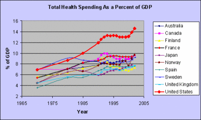
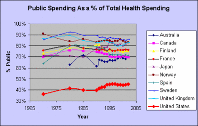
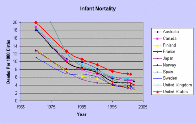
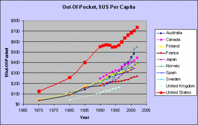
Professor Thoma's collection includes reference to a series of charts posted by Angry Bear between April 11th and April 25th, 2005 on the subject of health care. You can find the first Angry Bear post here, or the month of April 2005 Angry Bear archives here, or you can find the series of seven posts under the left hand column TOPIC heading for The U.S. Health Care System on Angry Bear's home page.

The four samples at the beginning this post give you a flavor of what's in store for you when you link back to Angry Bear's original posts and graphs. These are clear graphs that quickly deliver information that you may have heard about (e.g. U.S. infant mortality is high) but are not likely to have seen in such a visually powerful format.

Here's what I like about these posts individually and collectively.

1. The long and consistent time frame used for each chart stretching back to 1970.

2. The unusual readability given that Angry Bear is showing 10 different time series in each chart. The behavior of the U.S. series in red is especially easy to see in relation to the other countries' trends

3. The range of different metrics presented by the composite set of charts - in addition to the ones shown hear, there are charts for

+ Doctors per 1000 people,
+ Hospital Beds per 1000 people,
+ Life Expectancy at Birth,
+ Percent of Population over 65,
+ Percentage of Health Care spending for pharmaceuticals.

There are 10 separate interdependent metrics covering 35 years for 10 different countries.

4. The way that even a single chart such as the infant mortality trends could tell a story all by itself without any accompanying text (and having done so trigger the viewer to begin thinking more deeply about the meaning and underlying causes). This is not to say that a single metric is ever likely to be sufficient, but a good chart is sure a good way to start.

5. The nice integration of textual explanation in relatively close physical proximity with the related graphics.

In my opinion, Angry Bear's approach is a model to follow when addressing any important topic. The clear graphics covering multiple metrics and the accompanying text make excellent use of time series data to help make better sense of the complex topics of health care. At the same time this series encourages deeper thinking, and fosters further communication.

Angry Bear consistently produces excellent time series graphics and text dialogue on a range of interesting and important subjects. Repeating what I said earlier about Professor Thoma, it's definitely true that a careful study of Angry Bear's archives will provide many other examples of how best to harness the potential of time series graphics.

Check it out for yourself.

Note: this post was updated August 4th, 2005 at 5:28 PM with some corrections and additional material detail.

Timelines on the Web - Part VI - A Treasure Trove of Recent Graphs

Over the at Professor Mike Thoma's Economist's View, I have discovered a literal treasure trove of recent timeline graphics. My hat is off to Professor Thoma.

You can find this great assemblage at: Economist's View: Graphs.

Warning, this web page is about 8 MB and can take a while to load even on a high speed link.

However, if you are interested in seeing a wide range of examples of the ways different contributors on the web use graphics to present their points of view, this is a great place to start. Professor Thoma has included links back to the original postings where these graphs appeared to sites such as Angry Bear, Calculated Risk, Economist's View, Brad DeLong, Macroblog, New Economist, Econbrowser, The Big Picture, and Prudent Investor.

In total, there are over 300 pictures showing some of the most important metrics that impact our lives. For this collection, it's pretty clear than some bloggers are making good use of timeline graphics, can everyone else be far behind?

I plan on commenting on some of the best graphics in future post.

Thank you, Professor Thoma.

Timelines on the Web - Part V - Employment

Econbrowser: How many people should be working in America?

Professor James D. Hamilton's Econbrowser blog often provides excellent examples of the use of timelines to add to explanatory power and to promote conversation and collaboration around issues in our lives that affect us greatly.

His post a week ago on the recent scene regarding the employment situation in the U.S. is an excellent example of the ways that skillful use of time series graphics can add to the conversation and encourage further constructive conversation. [By the way, I call this TimeLine Collaboration (TLC) and one of the primary goals of this blog is encourage wider use of time series data in exactly this way.]

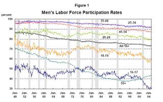
The trigger for the Econbrowser post was a Policy Brief written by Katherine Bradbury of The Federal Reserve Bank of Boston. Ms. Bradbury's brief is itself an excellent example of how best to make use of time series graphics to provide depth, breadth and insight to a complex topic.

Here's an example of one of her excellent and easily readable charts.




I plan to discuss her full document in more detail in a later post.








For now, I would like to focus on why I find Professor Hamilton's post on this subject so useful and helpful.

First, the post leads off with 9 links to others who have been commenting on the policy brief. This is really helpful for someone new joining the conversation.

"When Brad DeLong, Paul Krugman, Angry Bear, Economist's View, William Polley, VodkaPundit, The Big Picture, Lifelike Pundits, and Reading the World (among others)
all tell me to look at this policy brief by Katharine Bradbury, then, ok, I'll have a look at it."

Second, complementing the many excellent graphics in the policy brief, Professor Hamilton teases out three new time series graphs to dig deeper into the more subtle aspects of the question at hand. The graphs punctuate and support the arguments he makes with words. And the graphs themselves are easily readable and clear and quickly tell their story.

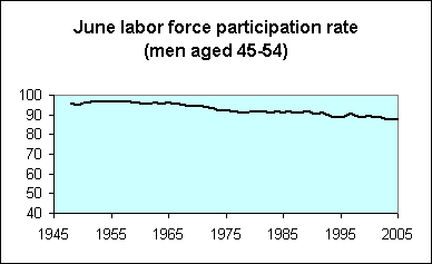
Here's one example where he draws out a single series from the policy brief figure 1 to help bring it more to our attention:

Note: I would have preferred to see this graph scaling from about 80 to 100 (rather than 40 to 100) on the Y axis to help visualize the trend more clearly. With a different Y axis scaling, the eye would be able to zoom in and detect trending over interesting sub-periods (e.g. the past 5 years). Right now, that kind of information is rather hard to read directly from this chart.

Professor Hamilton's blog directly includes timeline graphics with much greater frequency than many of the other popular economics blogs on the web. For example in following the 9 links for those who commented on the policy brief (and following further links from these 9) , embedded time series graphics were few and far between.

The text at these links was commenting on important metric after important metric and on their relationship, but it was the norm that there was nary a picture to clarify and reinforce the words. What a pity.

My view is that the inclusion of more pictures like those in the original policy brief and like those in Professor Hamilton's post will promote more and better conversations and understanding.

My open question to those who comment so regularly on matters economic is

WHY SO FEW GRAPHS?

I cannot imagine these economic experts coming to their conclusions or formulating the gist of their analyses in words without actually having looked at the time series that best inform the question at hand. When they show us their conclusions without at least showing us a few key pieces of the data upon which these conclusions were made, how does an impartial observer evaluate their work?

In fact, how can evaluation of any theories or hypotheses or explanations offered by these economics experts even be possible without looking at some of the data?

Since our own time is often the scarcest resource that determines what gets done and what doesn't, the lack of supporting charts in these posts (where the chief content is interpretation in the trends) effectively rules out proper evaluation in most cases.

What's left is whether we TRUST the writer or not. Not a good recipe for communication, collaboration and learning together about the things that matter most.

We will return to questions such as these in future posts.

Timelines on the Web - Part IV - Iraq Electricity

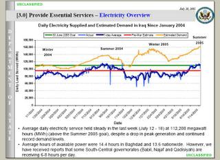
Here's the situation in Iraq with Electricity Demand and Current Generating Capacity.



It comes from the Iraq Weekly Status Report dated July 20, 2005 at: http://www.defendamerica.mil/downloads/Iraq-WeeklyUpdate-20050720.pdf

The image there will be clearer than the one I have included with this post. Check out the whole document which includes some other informative time series graphs on building a solid foundation for progress in Iraq.

What other metrics would we need to look at if we were to have a good feel and understanding for what is happening on the ground in Iraq?

COMMENTARY

I find the electricity chart to be clear and readable and readily understandable. What would make this data even more interesting would be to see what these same metrics looked like going back to 1980. Then, we could put the current demand and output in better perspective.

How does this report compare with what we are seeing on the Evening News?

Timelines on the Web - Part III - Criminal Justice

Key Crime & Justice Facts at a Glance

Here's a useful example of how a very complex domain of interest (Criminal Justice) can be represented as a series of time series pictures that highlight some of the important factors at work.

http://www.ojp.usdoj.gov/bjs/pub/pdf/charts.pdf

It's a set of 13 attractive and easy to read time series graphs all combined in a single PDF file for easy distribution. This PDF includes information about crime rates, prison populations, expenditures and so on.

DETAILS

This particular example includes factors such as:

1. violent crimes committed
2. violent crimes reported
3. arrests for violent crimes
4. property crime rates
5. crime rate by gender of victim
6. drug abuse violations by adults
7. drug abuse violations by juveniles
8. the homicide rate per 100,000 population
9. rape rates per 1,000 persons over 12 years old
10. violent crime by perceived age of offender
11. homicide by age of victim
12. correctional populations by jail, parole, prison, and probation
13. state prison population by offense type
14. prisoners on death row
15. executions
16. direct expenditures by level of government

Back at the Department of Justice, Bureau of Justice Statistics web site, at http://www.ojp.usdoj.gov/bjs/dtdata.htm you can find all these important metrics and literally thousands more.

For example, you can download a CSV file on reported crime from http://bjsdata.ojp.usdoj.gov/dataonline/Search/Crime/State/DownCrimeStatebyState.cfm/CrimeStatebyState.csv

COMMENTARY

While these pictures don't tell you everything you might ever want to know, they certainly are more than sufficient to begin an interesting and useful conversation about the trends in the area of Criminal Justice.

The domains of interest that most impact our lives are often complex and can only be understood by examining all of the most important factors in some detail to see how each of these changes over time. This particular presentation is in my opinion an excellent example of how to begin a conversation on these important topics.

As an alternative way to skillfully jump start a conversation, the related web page at: http://www.ojp.usdoj.gov/bjs/glance.htm provides a slightly larger set of charts in thumbnail format.

The thumbnails can be clicked through larger size image and some background infomration on that set of metrics. The larger size image can in turn be clicked through to see the underlying data.

The "At A Glance' page has the added bonus of providing a brief, 25 word or less statement about each thumbnail graph to help put it into context. E.g. "Serious violent crime levels declined since 1993."

All in all, I find this an excellent example and a skillful approach to presenting a complex subject. An ordinary person with no special expertise in Criminal Justice, Statistics, or Programming but moderately proficient at browsing the web can quickly become informed about the top level trends in Criminal Justice in the United States. And if time and interest permit, that same person can use that web site as a jumping off place for further in depth investigations.

ATTRACTIVE VISUAL FEATURES

Returning to the PDF file, it displayed a number of attractive visual featues that made this series of graphs much easier to read, interpret and digest.

A. The scales on the X and Y axis were extremely easy to read

B. For graphs with multiple series, they were very clearly labeled by attaching the text near the timeline trend which made it easy to figure out which series was which.

C. The number of metrics shown on a single graph was kept to reasonably small number (maximum of 4) which also added to readability. Colors were chosen so each metric was readily distinguishable.

D. Many, but not all, of the graphs used the same date range (1973-2001).

E. The individual graphs frequently included a detailed caption at the bottom that added to the total understanding.

F. Font size all around was very readable on a laptop screen, even when the window was reduced to 1/3 the size of the screen.


WHAT MIGHT HAVE MADE THESE EVEN BETTER

1. Providing a URL in each case that pointed to the source data

2. Organizing the sequence so all the charts covering the same time period were together

3. Including a 25 word or less comment in a prominent position similar to the ones that appear with the thumbnails on the AT A GLANCE page.

4. Having data that is more up to date. This is the most serious flaw in the data available on the PDF and on the AT A GLANCE page. The thumbnails show data through 2003, while the PDF only goes to 2001. If you are interested in Criminal Justice, you probably want to know what happened in 2004 and even in the first 6 months of 2005.

5. Some of these metrics might benefit from being observable as a monthly time series in addition to the the yearly view.

LATE DATA & EARLY WARNING SYSTEMS

Late data can be a serious impediment to proper understanding, especially if you are considering making decisions or interventions today based on the available data. By definition, when data is late, early warning goes out the window. The technology exists today to make this kind of data available in near real time, but in many real world cases, we are finding that really important data is unbelievably late.

We will return to this problem of late data later posts with some ideas on how to best deal with it.

Professor Pollkatz Speaks

Here's some more insight and clarity from Professor Pollkatz who we mentioned in an earlier post.

Check out page 6 of his "Footnotes" PDF where he defends his "fair use" right to use Gallup polling data in creating some uniquely powerful graphics.

http://www.pollkatz.homestead.com/pollkatzfootnotes02july.pdf

I particularly resonated on the following (emphasis added):

My graphics are informative in a way that mere data is not. The information the graphics provide is priceless, illustrating truths about vital public issues that otherwise might go unobserved and displaying those truths for all to see. Any number of people whose eyes might glaze over at columns of numbers or bar charts can read my graphics and understand their significance. Among other things, this reduces the power of unscrupulous journalists and public figures to “lie with statistics.” The graphics are also put to use, by me and others, to offer commentary and criticism on issues of public importance.

...

My graphics, by setting poll results on the same axes so they can be compared and contrasted, illustrate many things that single graphs would leave obscure. Foremost, depicting all the facts together shows broad trends that the vagaries of sampling hide in a single series. Also, viewers of the graphics can follow the relative position of a single poll organization, and decide for themselves whether that pollster exhibits any consistent biases. Omitting any pollster’s data from the graphic would diminish these values, let alone omitting Gallup, the most prominent pollster of all. It would be akin to leaving some neighborhoods out of a regional telephone directory.

I have compiled the data into a database, myself, from public sources. Converting the data to graphics has involved a considerable amount of programming skill (Microsoft Excel), and the Excel macros may themselves be copyrightable. People have written to me asking for help in doing similar graphics on other topics. By any standard, this qualifies my graphics as derivative works.

COMMENTARY:

For me the text "that otherwise might go unobserved" is the fundamental reason for looking for the best possible way to represent numeric time series data in some creative visual format so that all can see.

When done well, this transformation from eye glaze over data to potent pictures definitely has the power to reduce the ability of the unscrupulous among us from spinning stories that are contrary to the underlying facts.

When done brilliantly and creatively as Professor Pollkatz has done in this one small but important domain, it opens up the possibility of communication, collaboration, and greatly enhanced understanding of the factors that most affect our lives.

While moving in this direction may seem conceptually easy, the behind the scenes mechanics of acquiring the data and making it usable represent a serious impediment to our collective ability to transform the data into socially productive forms. This is exemplified with Professor Polkatz statement that "converting the data to graphics has involved a considerable amount of programming skill".

This is a key challenge not just for Professor Pollkatz' polling data but with time series data representing the most important factors in any domain of interest. There are an astronomical number of publicly available and vital data series. Many of these can be readily downloaded on the web.

For example, there are countless possibilities available from the Department of Labor, Department of Labor Statistics at: http://www.bls.gov/data/home.htm . And this web site makes all the data available and provides some powerful built-in capabilities for looking at individual time series. However, if you want to create a composite graphic that was not already designed into their reporting and graphing engine, you are on your own and the job is likely to be complex and time-consuming.

In subsequent posts, I will be addressing the specific question of the scarcity of our personal time and the complexity of the data. The goal will be to develop and refine a methodology and approach that makes the transformation from complex data to powerful time series graphics easier and easier.

If you want to change the world, build better tools.

Timelines on the Web - Part II

The Carpetbagger Report � A Reagan legacy - the world's leading jailer

Here's another excellent time series example recently posted on the web by Professor Ed Stephan. For me, Professor Stephan's timeline graph had immediate and visceral impact that fully supported the text portion of the posting.

The immediately obvious shape tells a powerful story about the dramatic changes that have taken place in the U.S. incarceration rate in the past 30 years. I found the red line data on the rate of prisoners per 100,000 population to be especially striking.

One thing that I like about this posting is that it also includes a direct link to the source data in Excel spreadsheet format. This opens the door to anyone interested to delve more deeply into the underlying Census Bureau data at HS-24: Federal and State Prisoners .

Sharing the data so easily in this way makes the possibility of conversation and collaboration between interested parties just so much more likely. Metaphorically, we might think of this as getting the best of two familiar ideas - a picture is worth a thousand words coupled with a journey of a thousand miles begins with a single step. When shared in this way, the data behind the picture can be come the sustenance for a shared journey by two or more parties leading in the end to deeper understanding.

Professor Stephan's regular guest posts at http://www.thecarpetbaggerreport.com/ frequently offer other good examples of the power of timeline graphics to add to the story or to even tell the story all by themselves.

Timelines on the Web - Part I

Here is a recent timeline example that is well worth studying - a visually rich demonstration combining data from many semi-independent sources to create a powerful composite effect showing the week by week poll popularity of President George W. Bush.

http://www.pollkatz.homestead.com/files/pollkatzmainGRAPHICS_8911_image001.gif

Compare the richness of Professor Pollkatz' graphics with the traditional ways polling information is shared with us -- typically as a single data point from a single poll - completely divorced and cut off from any history or context.

So, for example, our ABC evening news might tell us that the popularity rating in late June was 48% in their most recent poll. Think about how much more can be discerned with the Pollkatz graphic that lets us examine all the other recent poll numbers and the evolving pattern over the preceding weeks and months.

You can find some more of the time-series work of Professor Pollkatz (Professor Stuart Eugene Thiel of Depaul University) at:

http://www.pollkatz.homestead.com/

Check out his Approval/Disapproval Spread chart. It's an excellent example of the power of deriving new and revealing time series by arithmetically recombining other time series - in this case calculating the SPREAD by subtracting the DISAPPROVAL value from APPROVAL value.